Chapter3 R and Rstudio

3.1 R, RStudio, Git and Github install.

For a quick start.
1. First Install apps and packages through Terminal (xcode with apple store).

brew install --cask r
brew install --cask rstudio

brew install git   
brew install --cask github  

3.2 Git and Github tabs and commits.

For new projects, sometimes the git tab does not appear. In those occasions. Install:

xcode-select --install 

This solves the git tab missing problem.

In case the tab is still missing and there’s a need to do it manually. Check settings by going to:
// Tools > Version control > Project Setup > ...[]... > Git/SVN > Version control system > Git

Also check:
// Tools > Version control > Project Setup > ...[]... > Git/SVN > Build Tools > Project build tools > Website

After setting, closing and restarting project will deploy the git tab and functionality.

If fails, another option is to download xcode from the apple store. This is a big app, it takes some time to download and

Install xcode from Apple Store. (nor nessesary, but if everything else fails.. try it.)    

3.2.1 RStudio access to Git and Github.

Important. Support for password authentication was removed on August 13, 2021. Please use a personal access token instead.
See here for more information.
If fatal error message: unable to access ‘https://github.com/MarceloRosales/Research_Notebook.git/’: The requested URL returned error: 403
Then, Create a personal access token.

From August 13, 2021, Github is no longer accepting account passwords when authenticating Git operations. You need to add PAT (Personal Access Token) instead, you can follow the below method to add PFA on your system.

Create Personal Access Token on Github
From your Github account, go to Settings => Developer Settings => Personal Access Token => Generate New Token (Give your password) => Fillup the form => click Generate token => Copy the generated Token, it will be something like ghp_sFhFsSHhTzMDreGRLjmks4Tzuzgthdvfsrta.

Then follow below method based on your machine:
For Windows OS
Go to Credential Manager from Control Panel => Windows Credentials => find git:https://github.com => Edit => On Password replace with with your Github Personal Access Token => You are Done.
For MAC OS
Click on the Spotlight icon (magnifying glass) on the right side of the menu bar. Type Keychain access then press the Enter key to launch the app => In Keychain Access, search for github.com => Find the internet password entry for github.com => Edit or delete the entry accordingly, (delete old password and copy/paste Token number instead) => You are done. for linux and more info.

3.2.1.1 Commit trouble shooting:

Saving and committing changes to github but github Page not updating?
> Commits will be saved in github but will not be reflected in githun pages. For pages to be updated, first build book (bookdow::gitbook) by clicking on “build Book” in the “Build” tab, this creates/updates hmtl files, THEN go to the git tab and commit to github. Reload page in browser and changes will be applied.

Old summary of steps

1. Set up Github account.
   
2. Import rstudio global settings (See 3.2)
   
3. Update packages, then copy / transfer packages from older computer/rstudio ( See 3.3 method 1)
   
4. Install xcode app, from the App Store.
   
5. Oppen xcope app and follow setting instructions.
   
6. IMPORTANT *In MBP20 there is a constant error of packages not updating:
   1.Git is not working after macOS Update xcrun: error: invalid active developer path (/Library/Developer/CommandLineTools.

The problem is that Xcode Command-line Tools needs to be updated.

Solution #1
1. Go back to your terminal and enter:

xcode-select --install

You’ll then receive the following output:

xcode-select: note: install requested for command line developer tools

Open Xcode You will then be prompted in a window to update Xcode Command Line tools. (which may take a while)
Open a new terminal window and your development tools should be returned.

Addition: With any major or semi-major update you’ll need to update the command line tools in order to get them functioning properly again. Check Xcode with any update. This goes beyond Mojave…

After that, restart your terminal

Alternatively, IF that fails, and it very well might…. you’ll get a pop-up box saying “Software not found on server”, see below!

Solution #2 See link here.

3.2.1.2 Commits are not been attributed (to me) and does not appear in the contributions graph in github page

From git page.

About commit email addresses

GitHub uses your commit email address to associate commits with your GitHub account. You can choose the email address that will be associated with the commits you push from the command line as well as web-based Git operations you make.

For web-based Git operations, you can set your commit email address on GitHub. For commits you push from the command line, you can set your commit email address in Git.

Any commits you made prior to changing your commit email address are still associated with your previous email address.

Setting your commit email address on GitHub

Setting your commit email address in Git

1. Open Terminal.
2. Set an email address in Git. You can use your GitHub-provided no-reply email address or any email address. git config --global user.email "email@example.com"
3. Confirm that you have set the email address correctly in Git: git config --global user.email email@example.com
4. Add the email address to your account on GitHub, so that your commits are attributed to you and appear in your contributions graph. For more information, see “Adding an email address to your GitHub account.”

# Some git preferences.  
git status
git config --list
# set git email
git config user.email "email@example.com"
# confirm emal
git config --global user.email

3.3 Rstudio global settings Export/Import. Configurations and settings..

After Installing R and Rstudio with homebrew, R studio settings are need. Doing it manually takes time and usually all changes are not performed.

For more information on RStudio Link to site.
From RStudio 1.3, the settings and configuration were overhaul.

User Preferences
All the preferences in the Global Options dialog (and a number of other preferences that aren’t) are now saved in a simple, plain-text JSON file named rstudio-prefs.json. Here’s an example:

    "posix_terminal_shell": "bash",
    "editor_theme": "Night Owl",
    "wrap_tab_navigation": false

The example above instructs RStudio to use the bash shell for the Terminal tab, to apply the Night Owl theme to the IDE, and to avoid wrapping around when navigating through tabs. All other settings will have their default values.

By default, this file lives in AppData/Roaming/RStudio on Windows, and ~/.config/rstudio on other systems. While RStudio writes this file whenever you change a setting, you can also edit it yourself to change settings. You can back it up, or put it in a version control system. You’re in control!

If you’re editing this file by hand, you’ll probably want a reference. A full list of RStudio’s settings, along with their data types, allowable values, etc., can be found in the Session User Settings section of the RStudio Server Professional Administration Guide.

\(\color{red}{\text{How to get to the file?}}\)
1. If file is hidden by attibute, Unhide all files with Command-Shift-PERIOD. (To hide the files again, press the same key shortcut).
2. Open Terminal> type open ~/.config/rstudio, this will open the a finder window showing the folder contaning the file, look for the file rstudio-prefs.json.
3. Examine the file and check if preferences correspond to the ones set in R preferences.
4. Then copy/paste the file in Rstudio of the new machine (save a copy of original file before replacing with old preferences or manually modified the file).
5. Restart R.

Transfer of R global settings successful!!

---

Rstudio Options

title: "R Notebook"
output: html_notebook | html_document | 

title: "Untitled"
output: html_document

title: "Untitled"
output: pdf_document

title: "Untitled"
output: word_document

---

3.4 Copy/Transfer the packages installed on one computer or R version to another using Scripts.

3.4.1 Method 1: (!THE ONLY METHOD THAT WORKED) USE THIS ONE!!!!!].

Link to site
Originally from [here] (http://stackoverflow.com/questions/1401904/painless-way-to-install-a-new-version-of-r-on-windows){target=“_blank”}

1. Run on old computer / r version (2015MBP)

# update, without prompts for permission/clarification
update.packages(ask = FALSE)

# Set working directory
getwd()
setwd() # "/Users/Marcelo-Rosales/Box Sync/Documents/R/Rmarkdown/"
getwd()

# List all packages and save in a file. save() command
packages <- installed.packages()[,"Package"]
save(packages, file="Rpackages")

2. Run on new computer / r version (2020MBP) txtcol()

# Set working directory
getwd()
setwd() # "/Users/marcelorosales/Box Sync/Documents/R/Rmarkdown"
getwd()

#Load list of packages and install.
load("Rpackages")
for (p in setdiff(packages, installed.packages()[,"Package"]))
  install.packages(p)

Check <- installed.packages()

Transfer of packages to MBP20 on 220812.

# Set working directory
getwd() # "/Users/marcelorosales/Box Sync/Niigata Uni Box/Experiments/Photoconvertible FP/Experiment Notebooks"
setwd("~/Box Sync/Documents/R/Rmarkdown") # "/Users/marcelorosales/Box Sync/Documents/R/Rmarkdown"
getwd()

#Load list of packages and install.
load("RpackagesMBP20_220812")
for (p in setdiff(packagesMBP20_220812, installed.packages()[,"Package"]))
  install.packages(p)

Check <- installed.packages()

# update, without prompts for permission/clarification
update.packages(ask = FALSE)

# Set working directory
getwd()
setwd() # "/Users/Marcelo-Rosales/Box Sync/Documents/R/Rmarkdown/"
getwd()

# List all packages and save in a file. save() command
packagesMBP20_220812_1333 <- installed.packages()[,"Package"]
save(packagesMBP20_220812_1333, file="RpackagesMBP20_220812_1333")

---

3.4.2 Method 2: Quick Way of Installing all your old R libraries on a New Device. DOES NOT WORK!!

Link here. To install all the libraries that I had installed in my previous laptop. I did the following:

Step 1: Save a list of packages installed in your old computing device (from your old device). !Warning Before saving file make sure you are in the right working directory and make sure you KNOW WHERE THE FILE IS STORED.

# Set working directory where the files will be store. 
 
installed <- as.data.frame(installed.packages())
getwd()
setwd("/Users/Marcelo-Rosales/Box Sync/Documents/R/Rmarkdown") # modify folder as needed.
write.csv(installed, 'installed_previously.csv')

This saves information on installed packages in a csv file named installed_previously.csv. Now copy or e-mail this file to your new device and access it from your working directory in R.

Step 2: Create a list of libraries from your old list that were not already installed when you freshly download R (from your new device).

installedPreviously <- read.csv(file.choose(), header=TRUE) # header = true, to avoid Error bad restore magic number. 
getwd()
setwd("/Users/Marcelo-Rosales/Box Sync/Documents/R/Rmarkdown") # modify folder as needed. 

baseR <- as.data.frame(installed.packages())
write.csv(baseR, 'baseR.csv')

toInstall <- setdiff(installedPreviously, baseR)

We now have a list of libraries that were installed in your previous computer in addition to the R packages already installed when you download R. So you now go ahead and install these libraries.

Step 3: Download this list of libraries.

install.packages(toInstall)

That’s it. Save yourself the trouble installing packages one-by-one all over again. LIES!!

---

Since the code above is not interactive, I modify to suit my needs.(DOES NOT WORK NEITHER)
Since the function choose.dir is only for Windows and not for Mac. I created a custom dir.choose function

Run this script in the old computer.

library(rstudioapi) # Need this package for the prompt windows.

# 1. Costume made function to choose a directory interactively.-----------------
dir.choose <- function() {
  system("osascript -e 'tell app \"RStudio\" to POSIX path of (choose folder with prompt \"Marcelo asks where to save the file.\")' > /tmp/R_folder",
         intern = FALSE, ignore.stderr = TRUE)
  p <- system("cat /tmp/R_folder && rm -f /tmp/R_folder", intern = TRUE)
  return(ifelse(length(p), p, NA))
}

# 2. Save the list of all the packages installed in my old computer (old device).
oldRpks <- as.data.frame(installed.packages())
outdir <- dir.choose()
filename <- showPrompt(title = " asks:", message = "Enter name of the file with out extension or special characters", default = "oldRpks")
  filename
# As .csv file.
  write.csv2(oldRpks, 
            file = print(paste0(outdir, filename, ".csv")),
            row.names = FALSE)

# 3. Copy the oldRpks to the new computer

Run this script in the new computer.

# 4.Create a list of packages from my new computer (new device), Since Rstudio installation is new, packages are the "basic packages that come form R". I will name the file baseRpks.
baseRpks <- as.data.frame(installed.packages())

# 5. Load the oldRpks file created in the old Rstudio into the new computer.
oldRpks <- read.csv(file.choose(), header=TRUE)

# 6. Then by subtract matching packages (setting the difference), the remaining list will be the packages that are not installed in the new computer. /
toInstall <- setdiff(installedPreviously, baseR)

# 7. Install the packages from the list.
install.packages(toInstall)

3.4.3 Old method used to transfer (DISCONTINUE).

Link to site

---

3.5 Interactive Plots using R Markdown Notebook.

Link to site

Using Normal ggplot graphics, is possible to add 3d interaction with the plotly package.

ggplot2 example

library(ggplot2)

a <- ggplot(iris, aes(x=Sepal.Length, y=Petal.Length, color=Species)) + 
  geom_jitter() +
  xlab("Gene Type") +
  ylab("GFP Mean Intensity") +
  ggtitle("Microscope images GFP intensity") +
  theme(plot.title = element_text(hjust = 0.5))

a

Using ggplotly with in ggplot2,

library(plotly)

ggplotly(a)

Plotly example

Here a Plotly R Open Source Graphing Library.
And R Figure Reference: Single Page. How are Plotly attributes organized?

# Using plotly
library(plotly)

fig <- plot_ly(iris, type="scatter",  x= ~Sepal.Length, y= ~Petal.Length, color= ~Species, mode="markers") 

fig

library(plotly)

mtcars$am[which(mtcars$am == 0)] <- 'Automatic'
mtcars$am[which(mtcars$am == 1)] <- 'Manual'
mtcars$am <- as.factor(mtcars$am)

fig2 <- plot_ly(mtcars, x = ~wt, y = ~hp, z = ~qsec, color = ~am, colors = c('#BF382A', '#0C4B8E'))
fig2 <- fig2 %>% add_markers()
fig2 <- fig2 %>% layout(scene = list(xaxis = list(title = 'Weight'),
                     yaxis = list(title = 'Gross horsepower'),
                     zaxis = list(title = '1/4 mile time')))

fig2

Export Plotly graphs into MS PowerPoint.

---

3.6 R Markdown

3.6.1 Introduction.

Markdown is a simple formatting syntax for authoring HTML, PDF, and MS Word documents. For more details on using R Markdown see http://rmarkdown.rstudio.com.

When you click the Knit button a document will be generated that includes both content as well as the output of any embedded R code chunks within the document. You can embed an R code chunk like this:

summary(cars)

##      speed           dist       
##  Min.   : 4.0   Min.   :  2.00  
##  1st Qu.:12.0   1st Qu.: 26.00  
##  Median :15.0   Median : 36.00  
##  Mean   :15.4   Mean   : 42.98  
##  3rd Qu.:19.0   3rd Qu.: 56.00  
##  Max.   :25.0   Max.   :120.00

---

3.6.2 Including/Excluding Plots

You can also embed plots, for example:

Note that the echo = FALSE parameter was added to the code chunk to prevent printing of the R code that generated the plot.

It is a way to edit text that can be converted in HTML, PDF, Word with the knit function.

1. Install markdown from CRAN and use.
   
2. See for markdown syntax cheat sheets.

Here a R Markdown: The Definitive Guide.
Includes information of Bookdown in chapter 12 and blogdown in chapter 10. R Markdown Cookbook.
Creating Websites with R Markdown.
Authoring Books with R Markdown.
Themes for R Markdown.
Using R Markdown Notebook.

Markdown has different options available:

1. As Document: HTML, PDF, Word.
   
2. Presentation: HTML (ioslides), IITML (Slidy), PDF, PowerPoint.
   
3. Shiny: Shiny Document, Shiny Presentation.
   
4. From Template: Interactive Tutorial, Reprex (lots of features), Reprex (minimal), GitHub Document (Markdown), Package Vignete (HTML).

Presentation in:

1. HTML (ioslides): HTML presentation viewable with any browser (you can also print ioslides to PDF with Chrome).
   
2. IITML (Slidy): HTML presentation viewable with any browser (you can also print Slidy to PDF with chrome.).
   
3. PDF (Beamer): PDF output requires TeX (MiKTeX on Windows, MacTex 2013+ on OS X, TeX Live 2013+ on Linux).
   
4. PowerPoint: PoverPoint previewing requires an istallation of PowerPoint or OpenOffice.

Shiny:

1. Shiny Document: Can create an HTML document with interactive Shiny components. Shiny Document Test01.Rmd
2. Shiny Presentation: Creates an IOSlides presetntion with interactive shiny components.

From Template:

1. Interactive Tutorial (learn)
   
2. Reprex (lots of features)
   
3. Reprex (minimal)
   
4. GitHub Document (Markdown)
   
5. Package Vignete (HTML)

---

3.6.3 Important Notes for easy typing in Rmarkdown.

Some of the code does not work the same in word_documents as in html_documents.

To create a new line or return, insert 2 spaces after the point or end of the line.

Be careful with the characters themselves, these characters (1.) ’’ are not the same as these (2.) ``.

1. Gives ‘word’; a simple quotation, the key is next to the return/enter in the English keyboard or in the shift+7 in the japanese keyboard.
   
2. Gives word; a format and background style, the key is in the top left side before 1 in the English key or in the Shift+@ in the Japanese keyboard.

Inline R Code
It is possible to show r script outcome inline with the text. For example, the line:

There were 50 cars studied

was created with the inline code format:

There were `r nrow(cars)` cars studied  

Plain Code Blocks: Use the three thicks (beging/end) to add plain code blocks, this are displayed in a fixed-width font but not evaluated. Use the option+command+i shortcut and delete the {r} heading to convert code section in plain code.

This text is displayed verbatim / preformatted  

For more help or references on Rmardown styles go to:
> //Help> Markdown Quidk Reference

Color text: you can use.

Roses are \(\color{red}{\text{beautiful red}}\), violets are \(\color{blue}{\text{lovely blue}}\).

To add color to text is a little more complicated.

Roses are $\color{red}{\text{beautiful red}}$,
violets are $\color{blue}{\text{lovely blue}}$.  

---

3.6.4 Keyboard Shortcuts

from <r-markdown> page.
Knowing R Markdown keyboard shortcuts will save lots of time when creating reports.
Here are some of the essential R Markdown shortcuts: ``

command	on a Mac	on Linux and Windows
To access shortcuts	Option + Shift + K	Alt + Shift + K
Assignment operator <-	Option + -	Alt + -
Pipe operator %>%	Cmd + Shift + M	Ctrl + Shift + M
Quick Copy and paste	Select section + Alt + Command + downArrow
Move word or section up or down	Select section + Alt + Up/Down Arrows
Jump to Top or End	Command + upArrow or Command + downArrow
Write in several lines at the same time	Alt+Command+ L-click lines
Wrap text or chunck with characters	Just select text of chunk to be wrapped and type
Insert a new code chuck	Command + Option + I	Ctrl + Alt + I
Comment/uncomment current line/selection	⇧⌘C	Ctrl+Shift+C.
Outdent	Shift+Tab	Shift+Tab
Knit Document (knitr)	⇧⌘K	Ctrl+Shift+K
Output in document in the format specified in your YAML header with. The “k” is short for “knit”!	Command + Shift + K	Ctrl + Shift + K

Next we’ll cover shortcuts to run code chunks. But before doing this it is often a good idea to restart your R session and start with a clean environment.

command	on a Mac	on Linux and Windows
Restart your R session	Command + Shift + F10	Ctrl + Shift + F10
Run all chunks above the current chunk	Command + Option + P	Ctrl + Alt + P
Run the current chunk	Command + Option + C or Command + Shift + Enter	Ctrl + Alt + C or Ctrl + Shift + Enter

knitr can execute code in many languages besides R. Some of the available language engines include: Code chunks with brackets {} will be run by R while kniting to display results.

• R
• Python
• SQL
• Bash
• Rcpp
• Stan
• JavaScript
• CSS
• Java
• Json
• Ruby

Code Chunks
The R Markdown file below contains three code chunks. You can open it here in RStudio Cloud.
You can quickly insert chunks like these into your file with the keyboard shortcut
Ctrl + Alt + I (OS X: Cmd + Option + I),
the Add Chunk command in the editor toolbar
or by typing the chunk delimiters {r} and.

---

3.6.5 TO PREVENT CODE RUNNING

Seems like it is better to use R notebook instead of R markdown.

When you render your .Rmd file, R Markdown will partially run each code chunk and embed the results beneath the code chunk in your final report.

In Rmarkdown: TO PREVENT CODE RUNNING, ERASE CODE BRACKES AND CODE TYPE, USE ONLY ``.

If you don’t want any code chunks to run you can add eval = FALSE in your setup chunk with knitr::opts_chunk$set().

{r setup, include = FALSE} knitr::opts_chunk$set(eval = FALSE) Ex. As shown graphs above.

summary(cars)

Code shown but summary table not shown.

A better way to do it is to add in the code@s chunk header the opptions:

echo=TRUE, eval=FALSE

---

3.6.6 Plots and Interactive plots.

Embed plots, for example can be stopped by eval = FALSE:
Code for the graphic is here but it is not shown.

Code nor plot shown

Note that the echo = FALSE parameter was added to the code chunk to prevent printing of the R code that generated the plot.

!Comment: while trying the “eval” command, this error happen…

!Error in parse_block(g[-1], g[1], params.src) : duplicate label 'setup' or 

Error in parse_block(g[-1], g[1], params.src, markdown_mode) : 
  Duplicate chunk label 'cars', which has been used for the chunk:
summary(cars)

Solution Change the “name of the code chunk”: {r cars} to {r cars1.}

Chunk Options
Chunk output can be customized with knitr options, arguments set in the {} of a chunk header. Above, we use five arguments:

• include = FALSE prevents code and results from appearing in the finished file. R Markdown still runs the code in the chunk, and the results can be used by other chunks.
• echo = FALSE prevents code, but not the results from appearing in the finished file. This is a useful way to embed figures.
• message = FALSE prevents messages that are generated by code from appearing in the finished file.
• warning = FALSE prevents warnings that are generated by code from appearing in the finished.
• fig.cap = “…” adds a caption to graphical results.

See the R Markdown Reference Guide for a complete list of knitr chunk options.

---

3.6.7 Bonus: R Markdown Cheatsheet

RStudio has published numerous cheatsheets for working with R, including a detailed cheatsheet on using R Markdown! The R Markdown cheatsheet can be accessed from within RStudio by selecting Help > Cheatsheets > R Markdown Cheat Sheet.

• rmarkdown-cheatsheet.pdf>.
• rmarkdown-reference.pdf.
• Cheatsheets_2019.pdf.
• rmarkdown-cheatsheet-2.0.pdf.
• 17.1 Use RStudio keyboard shortcuts.
  
• R Markdown.

---

3.7 R Notebook

R Markdown Notebook. When you execute code within the notebook, the results appear beneath the code.

Try executing this chunk by clicking the Run button within the chunk or by placing your cursor inside it and pressing Cmd+Shift+Enter.

plot(cars)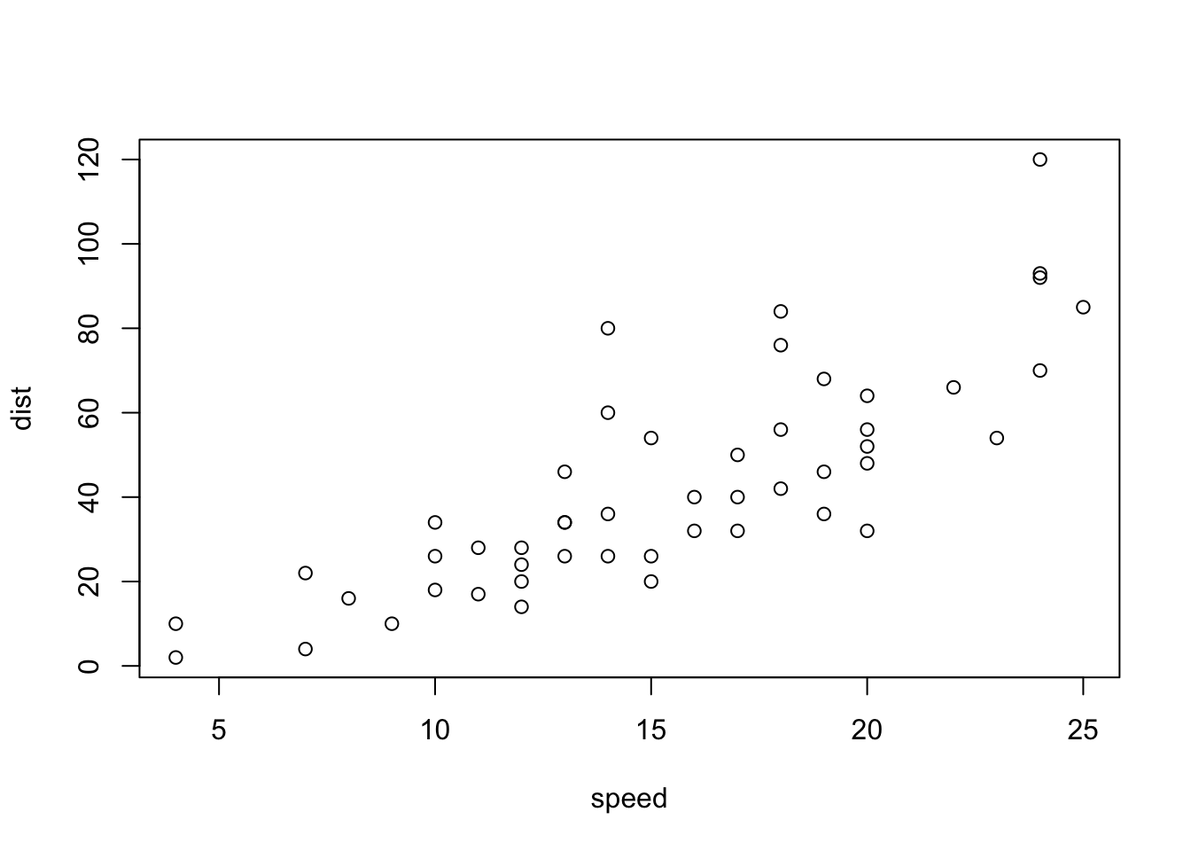

Add a new chunk by clicking the Insert Chunk button on the toolbar or by pressing Cmd+Option+I.

When you save the notebook, an HTML file containing the code and output will be saved alongside it (click the Preview button or press Cmd+Shift+K to preview the HTML file).

The preview shows you a rendered HTML copy of the contents of the editor. Consequently, unlike Knit, Preview does not run any R code chunks. Instead, the output of the chunk when it was last run in the editor is displayed.

A way to organize the Markdown text in section with the ability to preview the text without the need of knitting.
1. File> New file> Notebook.
2. To preview R Notebook, you have to save the file.
3. Once you saved the file, the preview will be available in the Viewer.
4. In the Meta-data leave the output as html_notebook.
5. And then start coding.

---

3.8 What is the difference between a Notebook and an R Markdown file?

Most people use the terms R Notebook and R Markdown interchangeably and that is fine. Technically, R Markdown is a file, whereas R Notebook is a way to work with R Markdown files. R Notebooks do not have their own file format, they all use .Rmd. All R Notebooks can be ‘knitted’ to R Markdown outputs, and all R Markdown documents can be interfaced as a Notebook.

An important difference is in the execution of code. In R Markdown, when the file is Knit, all the elements (chunks) are also run. Knit is to R Markdown what Source is to an R script (Source was introduced in Chapter 1, essentially it means ‘Run all lines’).

In a Notebook, when the file is rendered with the Preview button, no code is re-run, only that which has already been run and is present in the document is included in the output.

Also, in the Notebook behind-the-scenes file (.nb), all the code is always included. Something to watch out for if your code contains sensitive information, such as a password (which it never should!).

---

3.9 R Bookdown.

A way to manage several Rmad files and compile them in a gitbook style, with the possibility of multiple types of outputs, with support of figure/table number crossreference and can embed interactive content like HTML widgets/Shyny apps (if output is not html, take screenshots automatically) and compile as a gitbook.

Bookdown also can be uploaded to github where other collaborators can proof read and commit changes if nessesary.

DEMO for Authoring Books with R Markdown.

1. Download the GitHub repository Bookdown-demo as a Zip file, then unzip it locally.

2. Install the RStudio IDE. Note that you need a version higher than 1.0.0. Please download the latest version if your RStudio version is lower than 1.0.0.

3. Install the R package bookdown:

# stable version on CRAN
install.packages("bookdown")
# or development version on GitHub
# devtools::install_github('rstudio/bookdown')

4. Open the bookdown-demo repository you downloaded in RStudio by clicking bookdown-demo.Rproj.

5. Open the R Markdown file index.Rmd and click the button Build Book on the Build tab of RStudio.

---

3.9.1 Get started with bookdown

The easiest way for beginners to get started with writing a book with R Markdown and bookdown is through the demo bookdown-demo on GitHub:

1. Download the GitHub repository https://github.com/rstudio/bookdown-demo as a Zip file, then unzip it locally.
2. Install the RStudio IDE. Note that you need a version higher than 1.0.0. Please download the latest version if your RStudio version is lower than 1.0.0.
3. Install the R package bookdown:

• stable version on CRAN

install.packages("bookdown")

• or development version on GitHub
  devtools::install_github('rstudio/bookdown')
  1. Here, If you have other windows or projects running, in the right-upper corner of Rstudio main menu, there is a Project dropdown menu.
     
  2. Select Open project in New session.
     
  3. A new Rstudio window will open …[ ]…

4. Open the bookdown-demo repository you downloaded with RStudio by clicking bookdown-demo.Rproj. (Or through the Files Pane)
   
5. Open the R Markdown file index.Rmd and click the button Build Book on the Build tab of RStudio.

You can check the demo **A Minimal Book Example** in one window while still been able to work in the previews files or projects.

IMPORTANT!!: FOR ALL THE CHUNCK CODES ALWAYS USE: This will show the code but do not run it.

echo=TRUE, eval=FALSE

Also for “Helper Functions to Manage TinyTeX, and Compile LaTeX Documents” go to The R package tinytex/bookdown degging shoot

install.packages('tinytex')  

Update all your R and LaTeX packages:

update.packages(ask = FALSE, checkBuilt = TRUE)
tinytex::tlmgr_update()

---

3.9.2 R Bookdown tutorial quick start. (Latest update)

1. FIle > New project > …[]… > New Directory > Book Project using bookdown > Directory naem: -> Create project as subdirectory of: -> Browse ~/Documents/GitHub_Repos > √Open in new session … Create Project..
   
2. This will create all the files (.yml, book.bib, .Rproj, .text, .css, .Rmd, , including the “Index.Rmd which is the”initialization file” for the HTML book page. 8 file + 6 .Rmd).
   
3. Readme.md, _bookdown.yml, _output.yml and index.Rmd will automatically open.
   
4. In the **_bookdown.yml** file.
   1. Add output_dir: "docs" to create the docs folder for GitHub Pages.
5. In the _output.yml.
   1. Make sure the that the output is set to: bookdown::gitbook (the first line of the file).
      
   2. Additional outputs are set (pdf_book and epub_book). This automatically create this 2 formats as well as the HTML format. However; many times, this 2 outputs create conflicts in the building of the book, therefore I recommend to erase these formats unless they are need. In other words*:
      Erase the section:
      

   bookdown::pdf_book:  
     includes:  
    in_header: preamble.tex  
     latex_engine: xelatex  
     citation_package: natbib  
     keep_tex: yes  
   bookdown::epub_book: default  

   1. Change the title of the Book “before” and “after” names. In the sections <li><a href="./">A Minimal Book Example</a></li> to the name of the project, and in after, to any name you want.
      
   2. Save file.
      
6. In the index.Rmd file, make sure that in the YAML header:
   1. Site: ”bookdown::bookdown_site”
      
   2. Title: (change title).
      
   3. author: (change author).
      
   4. date: Change to: “Created: 2021/02/02, Latest update 2022-08-15”.
      
   5. description: (change description)
      
   6. Save file.
      
7. In Tools> Project Options …[ ]… > Build tools>, make sure that it is set to: website...
   
8. Since the project already started as a bookdown, the “build” tab will already be displayed in the Environment Panel. (See below if not).
   
9. Press the Build tab > Build book > bookdown::gitbook to create the bookdown page. (All Formats will create all the formats pdf and epub if available).
   
10. A new docs folders will be automatically created with all the html file needed for the web page. (**_book** and _bookdown_files folders are also created).
    
11. You can use the Knit button to preview the files.
    
12. Close the project, after configuration in GitHub app and GitHubPages, open again and project will display the Git Tab in the environment panel.

3.9.2.1 To conect/link new project to GitHub.

Go to the GitHub desktop app.
1. Go to the Repository List screen. (click in the down arrow next to Current Repository).
1. Click on Add (next to the Filter box).
1. Add > Add Existing Repository > …[]… Add local Repository > choose (Choose containing folder) > Open > …[]…
1. Message: This directory does not appear to be a Git repository. Would you like to create a repository here instead?
1. Click in Create a repository > …[]… Create a New Repository > √ Create Repository.
1. GitHub will create the repository in the app.
1. Then, √ Publish Repository > …[]… Un-check keep this code private > √ Publish Repository.

3.9.2.2 To create the website in gitHub Pages.

Go to GitHub.com page (browser).
1. GitHub.
1. In the repository list select the repsitory created.
1. MarceloRosales/Repo Name > Settings > GitHub Pages > Source > √ main > selected forlder: /docs > Save.
1. Your site is ready to be published at https://_.github.io//.
1. Close/Open Project(Repository) in RStudio and the Git tab will be displayed and available

---

3.9.3 R Bookdown tutorial quick start. (If not created as Bookdown)

1. File> New project> New directory> Empty project… [ ]… Directory name> choose location (subdirectory of…)
2. Once project is created, open a new R Markdown file: File> New File> R Markdown> Title of the book> Author > √HTML> OK
   
3. Save the new R Markdown document as ”index”. File will be saved as index.Rmd
4. Then in YAML header set:
   1. Output: ”bookdown::gitbook”
   2. Site: ”bookdown::bookdown_site”
   3. Save
5. Tools> Project Options …[ ]… > Build tools> set to: website..
6. Restart R project so R can recognize file as a book.
7. Once is restart, a build tab will be available in the Environment Panel.
   
8. [Build]> Build Book> … A gitbook will be created.
9. The index.rmd is the first chapter of the book.
10. To add another chapter create a new> R Markdown file> name chapter title. Ex. Chapter02
11. Then erase YAML and start with the chapter title with one single hash tag. Ex. # Hello World!
12. Rebuilt the book [Build]> Build Book> and the new chapter will be added.

To reference figures displayed by r code. In the fig code, place a name to the code chunck. Example

{r fig-name, fig.cap=’This is the figures caption and you can set the width, aspect, and align’, out.width=’80%’, fig.asp=.75, fig.align=’center’}
R code for figure

Then, reference the figure by its code chunk label with the fig: prefix, example.

See figure \@ref(fig:fig-name).  

†(In the Japanese keyboard option+¥ next to the backspace to make the backslash＼, but if Backslash is not set, go to symbol System preferences> keyboard> Input Sources> ‘¥’ key generates: Backslash. In word the ¥ key output is still ¥ but in Rstudio is .

For more information see Bookdown.org. There is Markdown/Bookdown syntax guide in Chapter 2 .

---

3.10 GitHub Pages and Bookdown:

3.10.1 Creating a booklike webpage with RStudio.

Hosting bookdown in github - Outline
Some packages may be required.

library(gh)

• Create bookdown in r in a “repository” folder.
• Add repository through github desktop.
• Close r bookdown and open again, (the git tab will appear)
• Add/Erase portions in the .yml files, build book and commit through R.
• Edit settings in github browser to show the web page from “docs” folder.

This method is a mix of other references but ultimately my experience to publish my bookdown to GitHub pages.

1. In RStudio, create a new bookdown project (in a new session) from template in a “repository” folder.
   • // Session > New Session
   • // New Project > New Directory > Book project using bookdown.
     
   • Choose Directory Name.
     
   • Choose the directory/folder to place the book project under. ( Do not use Box or Dropbox or Google Drive or any other cloud storage since RStudio is constantly creating and erasing file that could lead to conflicts when commiting a pushing.) The page will be saved in GitHub and version control will manage the updates in the folders/files. This is convinient, since all procedures will be made locally in the computer but committed and pushed to all computers/collaborator through Git.
   • A new book project will be created. All the files needed for bookdown web-page are automatically created.
2. Add the newly created repository folder to my GitHub account. Using the GitHub Desktop app.
   • Click on Current Repository
     
   • Click on Add.
     
   • Choose Add existing repository. This will Upload the repository created in the local folder to the GitHub account.
     
   • Add local repository path and click on Add Repository.
     
   • Some time will not recognize folder as repository. Click on create repository(?)
   • Commit by selection all files and filling the Summary box (required) and Push to GitHub. 1.　The Git tab: At this point there is no Git Tab in the environment Pane. Save the files in RStudio, and reopen the project and the Git tab in environment and Git button in main menu will be displayed.
     
3. Open the **_bookdown.yml** file and add output_dir: "docs" in a line.
   
4. Open the **_output.yml** file and erase this section from the file.
   

bookdown::pdf_book:
  includes:
    in_header: preamble.tex
  latex_engine: xelatex
  citation_package: natbib
  keep_tex: yes
bookdown::epub_book: default

This section creates a pdf and a e-pub files, but they constantly have problems building therefore is better to avoid them until needed.

5. Build the book buy clicking in //environment > Build > Build Book >
   
6. Check for Warning or errors in red, a successful creation should say Output created: docs/index.html, a new folder docs will be created containing all the html files for the page.
   
7. In //Environment > Git > Select all the files (cmmd + A) and check all files. Click on commit, place the commit comment and click commit.
   
8. Push all the files to GitHub.

---

3.10.2 To Publish the GitHub Page.

1. Go to the my GitHub account
   
2. In Repositories, choose the repository project created.
   
3. Go to Settings of the repository, scroll down to GitHub.
   
4. In source select branch: main and folder: /docs, then Save.
   
5. A new web address where the page is been hosted will be displayed.

---

3.10.3 Other method for Bookdown and GitHub Pages:

THESE METHODs PROVED TO BE MORE COMPLICATED, BUT ARE PLACE HERE AS REFERENCE. FOR A SIMPLER VERSION SEE GITHUB.

Video

---

3.10.3.1 Method 1. Existing project, GitHub first

Source; Happy Git and GitHub for the use R

A novice-friendly workflow for bringing an existing R project into the RStudio and Git/GitHub universe.
Probably your existing R project isolated in a directory on your computer. If that’s not already true, make it so.
Create a directory and marshal all the existing data and R scripts there. It doesn’t really matter where you do this, but note where the project currently lives.

1. Make a repo on GitHub. Go to https://github.com and make sure you are logged in.

   Click the green “New repository” button.
   Public
   YES Initialize this repository with a README.
   Click the big green button “Create repository.”
   Copy the HTTPS clone URL to your clipboard via the green “Clone or Download” button. Or copy the SSH URL if you chose to set up SSH keys.
   

2. Create a New RStudio Project via git clone

   In RStudio, start a new Project:
   File > New Project > Version Control > Git. In the “repository URL” paste the URL of your new GitHub repository.
   Suggest: “Open in new session”.
   Click “Create Project” to create a new directory, which will be all of these things:
   a directory or “folder” on your computer
   a Git repository, linked to a remote GitHub repository
   an RStudio Project
   This should download the README.md file that we created on GitHub in the previous step. Look in RStudio’s file browser pane for the README.md file.

3. Bring your existing project over

   Using your favorite method of moving or copying files, copy the files that constitute your existing project into the directory for this new project.
   In RStudio, consult the Git pane and the file browser. Are you seeing all the files? They should be here if your move/copy was successful.
   

4. Stage and commit
   

5. Push your local changes to GitHub

---

3.10.3.2 Method 2. Book down and GitHub Pages.

Source:.

1. In RStudio, create a new bookdown project (in a new session) from template.
   • // Session > New Session
     
   • // New Project > New Directory > Book project using bookdown.
     
   • Choose Directory Name.
     
   • Choose the directory/folder to place the book project under. ( Do not use Box or Dropbox or Google Drive or any other cloud storage. The page will be saved in GitHub and version control will manage the updates in the folders/files. This is convinient, since all procedures will be made locally in the computer but commited and pushed to all computers/collaborator throught Git.)
     
   • A new book project will be created. All the files needed for bookdown webpage are automatically created.
     
2. To Upload a bookdown to GitHub go to Terminal in Rstudio.
   

• In terminal See ‘git –help’.
  
• You can type:

git  # to see if  package is installed or not)
git –version # To the git version installed. 
git init  # Initialized empty Git repository in
git add . # add all
git commit -m”Add text file in case” # To add the comment in the commit. 

library(gh)
library(gitcreds)

Version Control with Git and SVN. (https://support.rstudio.com/hc/en-us/articles/200532077?version=1.4.1103&mode=desktop )
Setup for git in r https://r-pkgs.org/git.html.
From R, you can check if you already have an SSH key-pair by running:

file.exists("~/.ssh/id_rsa.pub")

Copy
If that returns FALSE, you’ll need to create a new key. You can either follow the instructions on GitHub or use RStudio. Go to RStudio’s global options, choose the Git/SVN panel, and click “Create RSA key…”:

In _output.yml erase bookdown::pdf_book: includes: in_header: preamble.tex latex_engine: xelatex citation_package: natbib keep_tex: yes bookdown::epub_book: default

In _bookdown.ylm add output_dir: “docs”

---

3.10.4 Bookdown Trouble shooting.

While installing R bookdown, there were several problems. To solve the problem:

1. Re-install all R packages from the package list of my 2015 MBP. (See 12.0.5 Script to copy the packages installed on one computer or R version to another).
   
2. Then update all packages with Update all your R and LaTeX packages command: (from 14.0.4)

update.packages(ask = FALSE, checkBuilt = TRUE)
tinytex::tlmgr_update()

1. Some error referred to the citr package and Latex. citr is the R zotero bibliography pack (see 14.0.7),
   
2. When building the page Make sure that the output is "bookdown::gitbook" and not in "All formats".
   
3. Other problem is the code chunks, RStudio will run all the code in the page unless specified otherwise. Therefore, Always use the {r eval=FALSE} at the beginning of the chunk code (echo=TRUE is the default setting, no need to type in)
4. Devtools packages did not installed correctly. Error: installation of package ‘devtools’ had non-zero exit status.

To solve this problem:

# 1st. try to Install devtools.
install.packages("devtools")

If devtools can not be installed. Install in terminal:

brew install libgit2

Then in R devtools and usethis packages.

install.packages("devtools")
install.packages("usethis")

Other packages that might be needed…

install.packages("cli")
install.packages("stringi")
install.packages("devtools")
install.packages("gert")
install.packages("git2r")
install.packages('usethis')

---

3.11 R and zotero for bibliography.

Install Zotero:

brew install --cask zotero

3.11.1 Zotfile

1. Download the zotfile-5.0.16-fx.xpi file from zotfile
   
2. In //Zotero > Tools > Add-ons > ‘Extensions’
   
3. Click on the gear in the top-right corner and choose ‘Install Add-on From File…’
   
4. Choose zotfile-5.0.16-fx.xpi just downloaded, click ‘Install’
   
5. Restart Zotero
   
6. //Zotero > Tools > Zotfile Preferences …[]…:

• General Settings > Custom Location: “/Volumes/MAR-NG-U/Zotero Data Directory/Zotero PDF’s”
  
• Renaming Rules:
• Renaming Rules original: {%a_}{%y_}{%t} changed to: {%a_}{%y}. Also {%b} which is used as a Wildcard for BetterBibTeX citekey (%b)
  
• Delimiter between multiple authors: old: &, new **_**.
  
• {%a_}= author last name; {%y_}=year; {%t}= Title; {%j}= journal

---

Guide/tutorial on using zotero in r

Install the BetterBibTeX plugin in Zotero and then use the citr package in R.
See here for General instructions on adding citations to an R Markdown document (though citr makes this easier):
Link here

Better BibTeX for Zotero.

• Highly customized exports.
  
• Fixes date field exports: export dates like ‘forthcoming’ as ‘forthcoming’ instead of empty, but normalize valid dates to unambiguous international format.
  
• Auto export of collections or entire libraries when they change.
  
• Pull export from the embedded webserver.
  
• Automatic journal abbreviation.

---

3.11.2 Start here: Zotero for R INSTALLATION

Installation instruction

1. Download the latest release of zotero better bibtex, make sure to save the XPI file, then in Zotero:
   
2. Open Zotero (standalone)
   
3. In the main menu go to Tools > Add-ons
   
4. Select ‘Extensions’
   
5. Click on the gear in the top-right corner and choose ‘Install Add-on From File…’
   
6. Choose .xpi that you’ve just downloaded, click ‘Install’
   
7. Restart Zotero

Note: the default setting of BBT will generate different citekeys that Zotero would itself generate; the keys from Zotero are not always safe for use in bibtex/biber. If you want to get the stock zotero keys, set the pattern in the preferences to [zotero]. I very much recommend not choosing [zotero] as your pattern unless you have existing articles that use keys generated by previous Zotero-native BibTeX export.

Once Zotero re-starts, set Configuration:

A welcome to better BibTex for Zotero will appear.(no longer appears junp to 1)
Select:
√ Use the BBT default format > Continue.
√ Enable darg-and-drop citations > Continue.
√ Unabbreviate journal names on import > Continue.
√ Expand (string?) journal names on imports > Continue.
All done.

3.11.2.1 Update 2021

1. Download the latest release of zotero better bibtex, make sure to save the XPI file, then in Zotero:
   
2. Open preferences: //Zotero > Preferences >…[]… Better BibTex.
   
3. Citation keys >

• Citation key format:[auth:lower][year];
• Keep citation keys unique: across all libraries.
  

1. Exports > Quick-copy > Pandoc; √ Surround Pandoc citation with brackets. (Gitbook? or LaTeX citation?)
2. Export > BibLaTex > √ Export unicode as plain-text latex commands.
   
3. Automatic export > √ On change.

---

3.11.3 For Zotero-R to work properly.

Open to Zotero Preferences>

To quick copy/paste form Zotero to Rstudio (command+ Shift +C). Set Config to Pandoc.
1. Zotero Preferences> Better BibTex> Citation keys>
a. Citation key format: [auth:lower][year]
b. Keep keys unique: √ Across all libraries.
c. Quick copy/drag and drop citations> QuickCopy format: √ Pandoc √ Surround Pandoc citations with brackets.
2. After that for easy export to Rstudio and Markdown, Go to:
Zotero Preferences> Export> Default Format: Better BibTex Quick Copy √

In Zotero> preferences> Better BibTex> Citation keys:

Default settings:
Citation key format: [auth:lower][year] QuickCopy Format: LaTex
LaTex command: cite for

Change to:
QuickCopy Format: Pandoc for (acar2015?)
√ Surround Pandoc citations with brackets.

Other Citation key format options: [auth:lower][shorttitle3_3][year]: ?
[zotero]: almeida_structural_2011
[zotero:clean]
[auth:lower][year]: alford2015 . IF duplicated alford2015a

Then I changed to [auth:lower][year][month]
For more cite configurations, go: Generating cite keys functions.

How to update all BibTex citation keys at once?
Select all, right-click, BBT->Refresh

---

3.11.4 To add Refereces/Bibliography to R bookdown.

1. Create a references.bib for the entire library (in zotero lib )
2. Select //Zotero > Mylibrary
   
3. //Zotero > File > Export Library…[]… > Format: Better BibTeX†; Translator option: Keep updated > OK …[]…
   
4. [Export] > Where: (MPB20-2021) /Volumes/MAR-NG-U/Zotero Data Directory/mylibrary.bib; Format: Better BibTeX > Save
5. Zotero will create the file
   
6. //Zotero > Preferences > Better BibTeX > Automatic export > Automatic export: On change (will change every time a new ref is added to zotero, this migth take several seconds). Others recomend Automatic export: Disable (Update of library will be made manually)

†Could also be BibLaTeX, see differences.

Watch this video as guide:

Steps

1. Add the references in the Markdown text with the quickcopy feature set above as in normal text. I advice to place all the related references in one folder in zotero, it doesn’t matter if you don’t use all the reference at the end. ex.
   [@almehmadi_vwc2_2018], [@rosales_rocabado_multi-factorial_2018].
2. In Zotero (standalone), select all the references you want to add.
3. Zotero// File> Export library.
   
4. Select Format: √ Better BibLaTex.
   
5. Check √ Keep update if you need to modify the bibliography in zotero, otherwise is not necessary.
   
6. Click ok/
   
7. Choose the namefile.bib and save inside the Bookdown Projects folder.
   
8. Chose Better BibLaTex and click Save.
   
9. In the index.Rdm YAML (Meta-data), add the name of the .bib file saved. bibliography: [book.bib, namefile.bib,]
   
10. Reference will be displayed at the end of the chapter after building the book.
    
11. To add an overall reference, Create a Reference.Rmd file and knit all references by typing the following code.

`r if (knitr:::is_html_output()) '
# References {-}
'`

1. Finally build the book and References will be created.

Here example of the meta-data YAML of Bookdown.

-- 
title: "A Minimal Book Example"
author: "Yihui Xie"
date: "`r Sys.Date()`"
site: bookdown::bookdown_site
output: bookdown::gitbook
documentclass: book
bibliography: [book.bib, packages.bib, myLibrarytest01.bib, Exported Items.bib]
biblio-style: apalike
link-citations: yes
github-repo: rstudio/bookdown-demo
description: "This is a minimal example of using the bookdown package to write a book. The output format for this example is bookdown::gitbook."
---

Examples and further reference here

---

3.11.5 Referencing a Figure

See here for details

---

3.11.6 To automatically create a bib database for R packages

# automatically create a bib database for R packages
knitr::write_bib(c(
  .packages(), 'bookdown', 'knitr', 'rmarkdown'
), 'packages.bib')

---

3.11.7 Example from the “Introduction” file in bookdown.

You can label chapter and section titles using {#label} after them, e.g., we can reference Chapter \@ref(intro). If you do not manually label them, there will be automatic labels anyway, e.g., Chapter \@ref(methods).

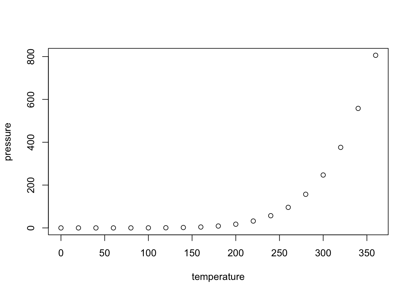
Figures and tables with captions will be placed in figure and table environments, respectively.

par(mar = c(4, 4, .1, .1))
plot(pressure, type = 'b', pch = 19)

Reference a figure by its code chunk label with the fig: prefix, e.g., see Figure 1.1. Similarly, you can reference tables generated from knitr::kable(), e.g., see Table 1.1.

knitr::kable(
  head(iris, 20), caption = 'Here is a nice table!',
  booktabs = TRUE
)

You can write citations, too. For example, we are using the bookdown package (Xie 2022) in this sample book, which was built on top of R Markdown and knitr (Xie 2015).

---

3.12 Blogdown.

Creating Websites with R Markdown.
Best R Hugo Blogdown Site End to End Tutorial Use this video as a guide.
Live-Tutorial Making Live Site, Blogdown Hugo GitHub Netlify Error at the end and did not deploy the site.
Video01.

1. Installs in Rstudio

2. Since blogdown is based on the static site generator Hugo Themes, you also need to install Hugo.

   While installing Hugo, check which Hugo version is been downloading.

3. Git and Github are also necessary. Install both.

   Git
   In git it is important that the “Git from the command line and also from 3rd-party software” is check. Actually it is the default setting so… not really necessary to do anything.

   In Github
   Signup/Login to github
   https://github.com/login
   MarceloRosales

   pw:token (1 year)

   mail:(hotmail.com?)

   In github create a new repository. (you can do it in terminal as well is much faster)

   MarceloRosales/Blogdowntest01
   add a Readme file.
   Create repository

   Once created, click in Code green button, and copy the “Clone” https URL link.
   https://github.com/MarceloRosales/Blogdowntest01.git

4. Once All installed is recomended to re-start Rstudio.

5. Next Create a New Project> Version Control> Git> Paste github URL to repository and assign a sub-folder to keep all site under the ”R Blogdown”** sub-directory. ( browse> ~Box/…/R Blogdown, R creates directly the folder name with the name of the repository)
   †If Rstudio is alread open and dont want to close the current windows/session, in the upper left corner of menu, select “Open project in new session”

6. Once the project is created, a new Git tab will be available in the Environment tab.
   

7. Go to the Hugo Themes and choose a theme.(Check is maintained or actively updated)
   

8. For this example I choose Airspace, Minimal, Health Science Journal. (Some theme require pay for extra features.)
   

9. CLick in Home page or download. This will redirect to the github repository
   

10. Copy the repository name: themefisher/airspace-hugo. (not the adress https://github.com/themefisher/airspace-hugo.)
    

11. In R create a new site with: †WARNING: Run this code in the blogdown project CONSOLE?, if run in other folder it may override files.

blogdown::new_site(theme = "themefisher/airspace-hugo")

1. All the files required will be created, and a preview of the site will be available.
   

2. In the console panel check for the virtula IP address or virtual host. ex, Serving the directory . at http://localhost:4321
   

3. Copy http://localhost:4321 paste in the browser and it should work as a webpage. The site is generated by R, so it is not deployed or uploaded to github.
   

4. WARNING: now that files are created. DO NOT change of replace the public folder.
   

5. In console; info and commands to start stop server are written.
   ― The new site is ready
   ○ To start a local preview: use blogdown::serve_site(), or the RStudio add-in “Serve Site”
   ○ To stop a local preview: use blogdown::stop_server(), or restart your R session
   

6. Next Stop the local server. To stop it, call blogdown::stop_server() in console or restart the R session. (in the video servr::daemon_stop(1))

   blogdown::stop_server()

7. Stage all files to github, for this use // Tools>Shell, seems like works better than Terminal.
   

8. In terminal set git user name: git config --global user.name "MarceloRosales"
   

9. In terminal set git user mail: git config --global user.email "selasorolecram@hotmail.com"
   

10. Stage all files: git add -A
    

11. Then in R Environment> Git> Commit …[]…, To Commit all files.
    

12. In Commit message type a description of the commint. ex. First commit.
    

13. Once all is committed, press close.

14. Then, click Push in the same window.
    

15. An error occurred… remote: error: GH007: Your push would publish a private email address. To solve:

    1. Go to Setting your commit email address.
       
    2. Follow the Setting your email address for every repository on your computer.
    3. Open your GitHub account, and go to Settings → Emails.
    4. Select the Keep my email address private check box.
    5. Unselect the Block command line pushes that expose my email check box.

16. Then, click Push in the same window again. Push successfull.

---

3.12.1 Setting Netlify.

Netlify.

Singup. With github. name: Marcelo Rosales

1. Click new site from Git.
   
2. Will ask for permision to acces github.
   
3. Select the repository to use.
   
4. Show advance.
   
5. Make sure Build command: hugo
   
6. Publish directory: Public.
   
7. Create New variable.
   
8. in key: HUGO_VERSION. (All caps).
   
9. In Value, type the hugo version. to see hugo version:

blogdown::hugo_version()

1. Click on Deploy site.
   
2. click on Preview
   
3. Warning It does not deploy correctly.
   
4. Go back to Site overview> Domain settings> Domains> Options. Here you can change the name of the domain to a more easy one. But if choose, you can not use that name EVER again.
   
5. To FIX the problem, copy the domain name link, (competent-montalcini-1e2438.netlify.app) and go back to RStudio.
   
6. Find the config.toml or config.yaml file and open.
7. Search for the baseurl and paste the domain name address. (https://competent-montalcini-1e2438.netlify.app/)
   
8. Save the file.
   
9. Stage the file (by checking the stage box).
10. Commit and Push.
    
11. Click on domain or paste link to web browser.
12. Success!! Page is live.

---

3.12.2 Creating websites in R with or with out blogdown using Jekyll.

Getting Started With Jekyll, The Static Site Generator

Like Hugo, is a website generator. That uses rmarkdown to generate html code.

To start a site got to jekyllrb.com:
Get up and running in seconds.

Quick-start Instructions:

gem install bundler jekyll
Jekyll -v
jekyll new my-awesome-site
cd my-awesome-site
bundle exec jekyll serve
# => Now browse to http://localhost:4000

Emily C. Zarbor post hass a nice guide.
Her webpage and Github are here.

Get Github Pages Site found in Google Search Results
You have to create a Google Search Console account and add your page, then typically you just drop a “marker” file in the root (Search Console generates this) so that Google can confirm you really own the page.

Google Search Console
Instructions

https://aksakalli.github.io/jekyll-doc-theme/ https://aksakalli.github.io/jekyll-doc-theme/docs/home/ https://bootswatch.com/3/ https://github.com/zabore/tutorials/blob/master/_site.yml

Jekyll themes
favorite theme:
TeXt Theme

---

3.12.3 Creating websites in R with blogdown and Hugo.

Hugogo.io

Defautl page: lithium, demo git page

Favorite Hugo themes:
Book, demo here
Bootstrap, demo here blog
Airspace, demo here
Zdoc, demo git page
Academia Hugo, demo git page
Dot, demo git page see the Inner Pages
Academic, demo no, but see Writing technical content in Academic Diagrams using mermaid, and sequence diagrams.
Andromeda Light, demo here
Tella, demo here
Restaurant Hugo, demo here
Timer Hugo, demo here
Hargo Hugo E-Commerce Theme, demo here
Parsa, demo here
Infinity, demo here
Navigator, demo here
Learn, demo git page
label, demo here
label, demo here
label, demo here
label, demo here

---

3.12.4 How to set a Hugo site with blogdown, modify and deploy using Rstudio.

3.12.4.1 Old version

Installs:
R
git
github
Rstudio
In Rstudio:
Blogdown

1. Create a git repository in github
   
2. Copy the clone or download repository key (https://github.com/….)
   
3. If git was successfully downloaded, a git tab should be present in the Rstudio environment section. If not after installing git, re-start Rstudio.
4. In Rstudio > New Project > Git > Clone git Repository > Repository URL:; Project directory name: > Create project.
   
5. Check the git tab is present.
   
6. Install blogdown package
   
7. Install devtools if necessary
   
8. Install Hugo themes blogdown::install_hugo()
   
9. Check Hugo version. blogdown.hugo.version = “0.88.1
   
10. Choose Hugo theme Hugogo.io see above for favorites.
    
11. Copy the theme’s github repository name
    
12. run blogdown::new_site(theme="name/ofrepository"
    
13. Hit enter and a new site will be created
    
14. Ones theme installed, the http://000.0.0.1:000 address will be created and displayed. Copy/Paste on browser and the site will be running on a local virtual host.
15. Type servr::daemon_stop(1) to stop virtual host.
    Commit and stage changes to git
    
16. Build page
    
17. set git version username git config --global user.name "github account name"
    
18. ser git version email git config --global user.email "github email address" (this will make sure your commits are registered under your name and appears in the panes in github)
    
19. Stage all files form build, type git add -A
    
20. In Rstudio click > “commit”, add comment > Push. 1.
21. Sign in Nitfly.
22. Create a new site
    
23. In Basic build settings make sure Build command = hugo > Publish directory = public.
24. Show advance > New variable > type: HUGO_VERSION > value: …0.88.1
    
25. If you don’t know value, Go back to Rstudio and in console type: **blogdown::hubo_version()** #0.88.1, copy/paste in value…
    
26. Deploy site (Netlify).
    
27. Netlify will build the site (Rstudion is not building the site), Netlify will search github for changes automatically
    
28. Then in Netlify set the domain or subdomain.
    
29. Then in Rstudio (build site), in the config.toml, search for the baseurl= “name of your domain”, build, save, commit and deploy, the site will be up and running.

3.12.4.2 New Versions

3.12.4.2.1 Installing the blogdown default (simple) website in minutes

Create site.
1. Install all dependencies. Blogdown, devtools, blogdow::install_hubo(), git, etc.
1. In rstudio > file > new project > new Directory > New Project > Directory name:… > create project as subdirectory of: … browse.. > create project.
1. in console type blogdown::new_site()
1. website is created, build and deployed in browser
1.

Modify site.
1. In the site files go to config.toml, you can make chages to the site here.
1. Create all new material in rmd files and save in the “content” folder.
1. Do not change public folder… unless you really know what you are doing.

3.12.4.2.2 Installing blogdown site using other hugo themes

1. Install dependencies and choose hugo theme (copy theme’s github repository name)
2. In rstudio > file > new project > new Directory > Website using blogdown > Directory name:… > create project as subdirectory of: … browse.. >
3. Uncheck the “convert all metadata to YAML” so we have the config.toml file instead >
4. Hugo theme:… (paste theme’s github repository name) > Create Project.
5. Click on Build to create the file of the website.
   
6. Serve/deploy the site with the code blogdown::serve_site
7. Once served, in console, a message with the site’s local ip is displayed. Copy/paste the address on a web browser if needed.
   
8. If there are issues with the site, stop the serving with the code servr::daemon_stop(1).
   
9. To modify content, go to site files and access the content folder and look for the rmd file of each page.
   
10. If you modify contents, press refresh on the brawser once to see changes, usually one refrech is need and after all changes are done automatically, making it really convenient while working on the content.
    

3.12.4.2.3 Modify blogdown hugo themes

---

3.12.4.2.4 Hugo structure

Blogdown site structure (as created with Rstudio)

• config: > **_default**: config.toml should be also here but it’s in root. To see the code documentation see here.
  • params.toml
  • menus.ko.toml
  • menus.en.toml
  • languages.toml
• content: All the content to be diplay in the website comes in this folder.
  
• layouts
  
• public
  
• R
  
• resources
  
• static
  
• themes: Here is were the Hugo template theme is going to be downloaded.
  
• index.Rmd
  
• ZdocTest1.Rproj: The name of the project and to open the project in Rstudio
  
• config.toml: This is the settings for the website.
  
• netlify.toml

---

Hugo Theme structure basically same as Hugo site created in R project

• archetypes: Data that helps you to find data about your content, ex. keyword or meta data.
  
• assets
• data: Act as a data base for your site. ex. jason files, etc.
  
• exampleSite
• i18n
• layouts: Here is were the information (HTML code) of how the website is going to look in general. Ex. footer for all pages (every single page). This folder contains:

  • index.html

  • _default:

  • blog

  • partials:

    • comments
    • drawer
    • footer
    • head
    • header
    • main
    • navbar
    • script
    • svgs

  • shortcodes

  • robots.txt

  • 404.html

  • index.json

• static: All the elements that do not change in webpage, ex. imges.
• LICENSE.md
• README.md
• theme.toml

└── themes   
    └── hugo-theme-zdoc     
        ├── LICENSE.md    
        ├── README.md  
        ├── archetypes  
        │   ├── default.md  
        │   ├── post.md  
        │   └── section.md  
        ├── assets   
        │   ├── js   
        │   └── sass   
        │       ├── abstracts    
        │       ├── layout  
        │       │   ├── _footer.scss   
        │       │   ├── _grid.scss   
        │       │   ├── _header.scss   
        │       │   ├── _main.scss   
        │       │   └── _navbar.scss   
        │       ├── main.scss   
        │       ├── pages   
        │       │   ├── _blog.scss   
        │       │   ├── _home.scss   
        │       │   ├── _list.scss   
        │       │   └── _single.scss   
        │       ├── syntax   
        │       └── themes   
        │           ├── _dark.scss   
        │           ├── _darkcode.scss   
        │           ├── _light.scss   
        │           ├── _lightcode.scss   
        │           └── _theme.scss   
        ├── data   
        ├── exampleSite   
        │   ├── config   
        │   │   └── _default   
        │   │       ├── config.toml     
        │   │       ├── languages.toml  
        │   │       ├── menus.en.toml   
        │   │       ├── menus.ko.toml   
        │   │       └── params.toml   
        │   ├── content   
        │   │   ├── en   
        │   │   │   ├── _index.md   
        │   │   │   ├── blog  
        │   │   │   │   ├── _index.md  
        │   │   │   │   ├── emoji-support.md   
        │   │   │   │   ├── markdown-syntax.md   
        │   │   │   │   ├── placeholder-text.md   
        │   │   │   │   └── rich-content.md   
        │   │   │   ├── docs   
        │   │   │   │   ├── _index.md   
        │   │   │   │   ├── contentfortmats.md   
        │   │   │   │   ├── contentmanagement   
        │   │   │   │   │   ├── _index.md    
        │   │   │   │   │   ├── frontmatter.md    
        │   │   │   │   │   ├── sections.md    
        │   │   │   │   │   └── shortcodes.md   
        │   │   │   │   ├── depth1    
        │   │   │   │   │   ├── _index.md   
        │   │   │   │   │   ├── depth2   
        │   │   │   │   │   │   ├── _index.md   
        │   │   │   │   │   │   ├── depth3   
        │   │   │   │   │   │   │   ├── _index.md   
        │   │   │   │   │   │   │   └── test3.md   
        │   │   │   │   │   │   └── test2.md   
        │   │   │   │   │   ├── test1.md    
        │   │   │   │   │   └── ttttest.md    
        │   │   │   │   ├── gettingstarted    
        │   │   │   │   │   ├── _index.md    
        │   │   │   │   │   ├── basicusage.md    
        │   │   │   │   │   ├── configuration.md    
        │   │   │   │   │   ├── installation.md   
        │   │   │   │   │   └── quickstart.md    
        │   │   │   │   ├── imageprocessing.md    
        │   │   │   │   ├── pagebundles.md    
        │   │   │   │   ├── pageresources.md    
        │   │   │   │   └── relatedcontent.md   
        │   │   │   └── updates   
        │   │   │       ├── 2019_april.md    
        │   │   │       ├── 2019_february.md    
        │   │   │       ├── 2019_january.md    
        │   │   │       ├── 2019_march.md     
        │   │   │       ├── 2019_may.md    
        │   │   │       └── _index.md    
        │   │   └── ko    
        │   ├── resources   
        │   │   └── _gen    
        │   │       └── assets   
        │   │           └── scss     
        │   │               └── sass    
        │   └── static     
        │       ├── favicon    
        │       ├── images    
        │       │   ├── landscape.jpg    
        │       │   ├── mountain.jpg   
        │       │   └── mountains.jpg    
        │       ├── logo.png     
        │       └── manifest.json     
        ├── i18n    
        │   ├── en.toml   
        │   └── ko.toml    
        ├── layouts     
        │   ├── 404.html    
        │   ├── _default    
        │   │   ├── _markup    
        │   │   │   ├── render-image.html   
        │   │   │   └── render-link.html    
        │   │   ├── baseof.html    
        │   │   ├── rss.xml   
        │   │   ├── section.html    
        │   │   ├── single.html    
        │   │   ├── sitemap.xml    
        │   │   ├── summary.html   
        │   │   └── taxonomy.html   
        │   ├── blog    
        │   │   ├── section.html   
        │   │   └── single.html   
        │   ├── index.html    
        │   ├── index.json    
        │   ├── partials    
        │   │   ├── comments    
        │   │   ├── drawer    
        │   │   ├── footer   
        │   │   ├── head    
        │   │   │   ├── meta.html    
        │   │   │   ├── meta_json_ld.html   
        │   │   │   ├── scripts.html   
        │   │   │   ├── services.html    
        │   │   │   └── styles.html    
        │   │   ├── header    
        │   │   │   ├── blog-header-img.html   
        │   │   │   ├── blog-header-text.html    
        │   │   │   ├── blog-header.html    
        │   │   │   ├── custom-header.html    
        │   │   │   └── site-header.html    
        │   │   ├── main    
        │   │   │   ├── component   
        │   │   │   │   ├── article-meta.html   
        │   │   │   │   ├── breadcrumb.html    
        │   │   │   │   ├── edit-this-page.html    
        │   │   │   │   ├── pagination-single.html    
        │   │   │   │   ├── pagination.html    
        │   │   │   │   ├── tag-cloud.html   
        │   │   │   │   ├── toc.html    
        │   │   │   │   ├── toggle-menu.html   
        │   │   │   │   └── toggle-sidebar.html   
        │   │   │   ├── header.html   
        │   │   │   ├── home.html   
        │   │   │   ├── landing    
        │   │   │   │   ├── home-landing.html    
        │   │   │   │   ├── home-sections.html    
        │   │   │   │   ├── home-social.html    
        │   │   │   │   ├── section-card.html   
        │   │   │   │   └── section-normal.html   
        │   │   │   ├── list.html   
        │   │   │   ├── sections     
        │   │   │   │   ├── list-main.html    
        │   │   │   │   ├── list-menu.html    
        │   │   │   │   ├── list-section.html    
        │   │   │   │   └── single-menu.html    
        │   │   │   └── single.html    
        │   │   ├── navbar    
        │   │   │   ├── icons    
        │   │   │   │   ├── light-dark-toggle.html   
        │   │   │   │   ├── navbar-icons.html    
        │   │   │   │   └── select-lang.html    
        │   │   │   ├── logo    
        │   │   │   │   ├── navbar-logo-mobile.html    
        │   │   │   │   ├── navbar-logo-tablet.html    
        │   │   │   │   └── navbar-logo.html    
        │   │   │   ├── menu    
        │   │   │   │   ├── navbar-menu-collapse.html    
        │   │   │   │   ├── navbar-menu-mobile.html    
        │   │   │   │   └── navbar-menu.html    
        │   │   │   ├── navbar.html    
        │   │   │   └── search    
        │   │   │       ├── site-search-mobile.html    
        │   │   │       └── site-search.html   
        │   │   ├── script    
        │   │   │   ├── codeblock-script.html    
        │   │   │   └── single-script.html    
        │   │   └── svgs   
        │   ├── robots.txt    
        │   └── shortcodes    
        ├── static   
        │   ├── fonts    
        │   ├── images    
        │   │   ├── header    
        │   │   │   └── background.jpg    
        │   │   ├── landscape.jpg   
        │   │   ├── mountain.jpg   
        │   │   ├── mountains.jpg   
        │   │   └── section   
        │   │       ├── keyboard.png   
        │   │       ├── processor.png   
        │   │       └── root-server.png   
        │   ├── logo.png     
        │   └── manifest.json     
        └── theme.toml    
        

---

3.12.4.3 Creating a Hugo Theme from scratxh.

See the original page here

# Create a new Hugo site
hugo new site example

# Create a new theme
hugo new theme exampleTheme

# starting the server
hugo server

# start the server including content marked as draft
hugo server -D

# Web Server is available at 
http://localhost:1313/ (bind address 127.0.0.1)

# to stop the server
Press Ctrl+C 

# create new file
touch filename

# delete file
rm filename

#  Create nes folder
mkdr dirname

# Delete folder
rm -r dirname

---

3.13 Useful Tips.

3.13.1 Math Formula inputs.

In the UI menu // n Add-ins menu, there is the Input LaTeX Math. Write the math formula and a latex source will be generated.

For example*.
a + ß = _{i=1}^nX_i.

Then add $ at the beginning and the end of the equation and formula will be display as a professional math formula in the preview.

\(x^2 + y^2\)

\(a\ +\ ß\ =\ \sum_{i=1}^nX_i\)

---

3.13.2 Displaying Code and Plosts

• Always use the {r eval=FALSE} at the beginning of the chunk code to stop RStudio automatic run.
  
• To have a better control on how to display the code chunks and plots, use the chunk Preferences. It appears in the Editor panel when {r} or other code type is at the head of the code chunk.
  
• Click on the gear icon and several option will be available.

---

3.13.3 How to add/embed videos and images.

Videos
To embed videos in markdown.

![](https://youtu.be/GAVXVkcpbG0){width="100" height="100"}.  

OR:

<iframe width="560" height="315" src="https://youtu.be/GAVXVkcpbG0" frameborder="0" allowfullscreen></iframe>  

knitr::include_url("https://youtu.be/GAVXVkcpbG0")

Images
To add a pictures, use:
source 01.

![Caption for the picture.](/path/to/image.png)

But this do not offer the ability to adjust the image to fit the page (see Update, below). To adjust the image properties (size, resolution, colors, border, etc), you’ll need some form of image editor. I find I can do everything I need with one of ImageMagick, GIMP, or InkScape, all free and open source.

Update:
Pandoc incorporated “link_attributes” for images. “Resizing images” can be done directly. For example:

The bookdown book does a great job of explaining that the best way to include images is by using `include_graphics()’. For example, a full width image can be printed with a caption below:

The reason this method is better than the pandoc approach ![your image](path/to/image) is because: - It automatically changes the command based on the output format (HTML/PDF/Word) - The same syntax can be used to the size of the plot (fig.width), the output width in the report (out.width), add captions (fig.cap) etc. - It uses the best graphical devices for the output. This means PDF images remain high resolution.

---

3.13.4 How to check Differences between rmarkdown files

The diff_rmd function can be used to produce a nicely-formatted document showing the differences between two rmarkdown files. This function can be used to compare two files, or a file with previous versions of itself (within a git repository). See here for more info.

You can install the development version of reviewer from GitHub with:

remotes::install_github("ropenscilabs/reviewer")

See the package vignette for a demonstration.

The diff_rmd function can be used to produce a nicely-formatted document showing the differences between two rmarkdown files. For the purposes of demonstration, we’ll use the example files bundled with the package. We’ll compare modified_file to its earlier version.

Reference_file:

modified_file <- system.file("extdata/CheatSheet-modified.Rmd", package = "reviewer")
reference_file <- system.file("extdata/CheatSheet.Rmd", package = "reviewer")

Compare:

library(reviewer)
result <- diff_rmd(modified_file, reference_file)

And our output:

We can also compare the current version of a document to a previous version in stored in a git repository.

If a reference_file argument is not provided, by default the modified_file will be compared to the most recent copy in the git repo:

result <- diff_rmd(modified_file)

Or we can compare it to how it appeared in the git repository after a particular commit (here, the commit with reference 750ab4):

result <- diff_rmd(reference_file, "750ab4")

---

References

Xie, Yihui. 2015. Dynamic Documents with R and Knitr. 2nd ed. Boca Raton, Florida: Chapman; Hall/CRC. http://yihui.org/knitr/.

———. 2022. Bookdown: Authoring Books and Technical Documents with r Markdown. https://CRAN.R-project.org/package=bookdown.